Real-time Semantic Image Segmentation via Spatial Sparsity论文笔记
由ypyu创建,最终由ypyu 被浏览 18 用户
这篇文章是针对real-time 图像分割做的工作,近期挂到arxiv上的。
最终的结果是可以在单独的GTX 980上每秒钟处理15张高分辨率cityscapes(1024*2048)的图片数据,同时在cityscapes测试集上保持72.9%的Mean IOU.
 这篇文章的主要贡献有两部分:
1.对于一个典型的两输入的全卷积网络引入了空间稀疏性,展示了在提高inference速度的同时并没有随时太多精度;
2.展示了使用空间稀疏性,使用in-column和cross-column的链接、移除残差单元,能够25倍的缩小计算开销,丢掉一点精度。
 这篇文章提出的架构是这种two-column的架构,接受两个输入,一个是full-resolution, 另一个是half-resolution的input。
最后prediction的时候,可以从这两个分支的 score maps来计算the element-wise sum/max; 或者生成scale-aware的权重,然后计算加权的element-wise sum。实际上half-resolution的计算开销只有full-resolution的四分之一。
这个模型的关键是low-resolution 分支生成的稀疏的weight map, 每个值都和原分辨率的square 的区域相关。如果在half-resolution 中的weight map是零,就表示这部分区域不需要被full resolution部分处理,half-resolution已经足够了。而且,通过不处理一些full resolution区域的部分已经足够补偿生成weight map的额外消耗。
 为了增大提取出的score map的分辨率,一直以来有三个比较典型的方法。1)典型的FCN,从不同resolution的feature map上预测score map,然后直接融合(sum)这些score map来做最后的prediction. 2) Deeplab移除了部分下采样的操作,使用空洞卷积来增大感受野,然而大的feature map就必然会导致计算开销的增大。3)也就是本文使用的,从SharpMask中引入的SharpMask结构,SharpMask最先是在instance Segmentation中提出的, 将low-level的特征和high-level的语义信息结合, 后面的实验也是表明了这种结构在效果和效率上有一个比较好的trade-off。
 在语义分割这样的task上,content的size经常是有很大变化的,这也说明了multi-scale处理的重要性。一个典型tow-column的pipeline分成三步: 1.计算原始输入大小image的score map;2.下采样image, 计算另一组的score maps; 3.把这两组score map合并到一起。
这张图片就是讲了muti-scale最后融合score maps的四种方法,1)最直接的两种放到就是做element-wise的sum/max;2) 另外一种方法是生成scale-aware weights的参数,然后用Softmax(then apply the Softmax activation function to ensure that the two entries at the same spatial location sum to one ),最后计算element-wise 加权的和,这种方法就是图中中间部分被称为 Attention-to-scale的方法。在Attention to scale那边论文中,被称为注意力模型,就是通过一个注意力模型来获得权重融合feature maps.最终得到分割的图像。
这个权重是怎么产生的呢?通过学习,对于每个尺度的特征图输出一个权重图。
这种方法的缺点就是依赖全分辨率和办分辨率两个分支上的 scale-aware weights 。
4)第四种就是本文用的,“coarse-to-fine’ approach ,scale-weight 仅仅依赖half-resolution的分支,通过卷积层去学习参数,然后经过sigmoid变为最后的weight。
 这里引入了对network产生的激活weights参数稀疏。最简单的想法就是winner-take-all策略,比如除了最大的k个激活值,其他全设成0.
另一种方法就是有一篇文章在受限玻尔兹曼机中提出的,去惩罚每个激活的分布的交叉熵,给定不同的输入data,以特定的概率p去激活。
我们希望这里一张图片的square区域会被赋予all-zero的权重值,这样就可以在full-resolution中跳过这些区域。
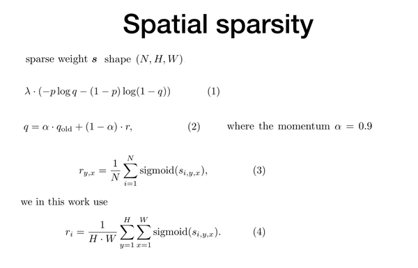
假设一张图片被分成H*W的square 区域,有t^2个vectors和每个区域相关。我们应用t*t的卷积核,步长也为t,然后就得到了H*W个元素的权重矩阵,每个元素都和feature map中的一个对应区域相关。假设每个batch有N个图片,然后我们得到的sparse weight s will have shape (N, H, W ). 为了保证稀疏,增加了term(1)式到loss function, lamudan 是这项loss的权重,p是指定的概率(手动设置的参数),q是移动平均概率。Qold is the moving average probability used in the previous iteration, r 只用当前表示概率估计. 注意本文中的r使用的是第四个eq. 在cityscapes这样的图片上通常都有一个特定的结构,比如在图片的上半部分有连续的区域(sky),或者在底部有另一种连续的区域(road).这表明一个区域的激活概率应该随着空间位置的改变而变化。因此,在本文中,没有用到第三个ep(每个location given一个可能概率来skip regions),而是用了第四个ep(每张图片given一个可能概率来skip regions).
第三个等式就是在一篇基于受限玻尔兹曼机提出的。
 这张图就表示了文章提出的架构。最后,计算一个scale-aware的weight maps. i.z. 对于half-resolution z1 ,对于full-resolution z2. 也计算一个稀疏的weight map s。
然后上采样s 到 z2的shape, 计算和z2两个element-wise的乘积, 这就是sparse ‘coarse- to-fine’ weight map required for the full-resolution column.
这个基本模型work的很好,但是丢掉了很多精度。这个问题的原因是an image is sliced into too small crops (typically 256×256) ,so a lot of pixels (near the boundary of an image crop) are classified without enough contexts during fast inference. 为了解决这个问题,又做了模型的两个改变。
1.we also crop each input image during training. 在inference的时候也crop 图像。这样使得train时候和inference的时候提取的特征是一致的。image crop分成不同的samples, 然后再把put their feature maps together to approximate those of the original image. 这种操作叫做“uncrop”.
2.加入cross-column connections,也就是在两个分支之间有连接。因为half-分辨率的column会覆盖全局的信息,在full-resolution分支上加入这些信息可以帮助缓解 the boundary problem。 We label this model as ‘improved sparse coarse-to-fine’.
这张图里面conv 3,128,3,8表示3*3卷积,128个kernels, 空洞卷积dilation rate=3,然后分成八组,分组卷积。蓝色的方形表示cropped input的feature maps; 红色部分表示只在训练中使用的; 绿色部分表示反传的梯度不会通过的区域。
First, we gradually reduce the number of kernels as the feature maps grow spatially, i.e., 128, 64 and 32. Second, we introduce group sparsity [13], i.e., eight groups for those layers directly on top of the raw features, and respectively eight, four and two groups for those 1×1 layers within the jump connections. Third, we use a 1×1 (but not 3×3) layer on top of the raw features in the full-resolution column.
文章也实验了移除resnet50的残差unit对结果的影响。
 在cityscapes上的实验;使用resnet50 MXNet.
恢复原始的分辨率有两种方法:1)up-sampling layers together with jump connections on top of the features. 2) 空洞卷积, 文中把这两个方法结合起来做了实验。
Table1表示了单column模型在效率和精度上trade-off的一个情况,最后选择了第三组,use three up-sampling layers with jump connections. 这三组实验都是sharp-mask结构的。
Table2表示了模型 two-column的不同融合方法在验证集上的效果。尽管计算量从165g to 206g, 增长了25%, IOU结果也确实有很大提升。
结果表明最后的scale-aware weight不必依赖full-resolution的那一个分支,这也是通过引入空间稀疏性加速inference的一个原因。换句话说,我们可以跳过一些full-resolution分支中input image的一些区域,来减少计算消耗。
SCTF: 增加稀疏性
ISCTF : 增加稀疏性 + the cross-column connections. 使用half-resolution的long-range context information 信息来增强full-resolution的features信息。
 Table3 这个表是针对空间稀疏性做的一系列对比试验,
开始due to the boundary problem,IOU从 74.72% 降低到了to 71.74%。
后来,applying the winner-take-all strategy. 也就是在那个weight map上选出最大的k个值,skip the same number of regions per image,分别是8,12,16个区域等等。
这里也做了 local regions 很小(变成128*128个regions时候),因为它很难克服边界问题,所以效果比较差。
最后的,在p = 0.5 , lamuda = 0.001时候,达到了75.4%的IOU.
 Table 4. 表示移除resnet50部分残差unit的结果。
最下面的这张图展示了计算消耗和一些components的贡献。
最后计算量从786—>31.5,缩小了25倍,only with a 0.6% loss of accuracy.
 和之前一些方法的比较。
speed tested in the built-in profiler of MXNet.
evaluated using a PC having one i7-4790 CPU and one Geforce GTX 980(1024*2048 size) video card installed with CUDA 8.0 and cuDNN 5.1.
Note that the speeds are only for reference, since the implementation details vary significantly between different works.
 一些效果,
一些效果,
Due to lack of context information, the SCTF model failed to identify some pixels inside the yellow car, while the ISCTF model is able to figure it out.
We also show two examples of the activated local regions in the full-resolution column in the third row.
there usually are small pedestrians or vehicles around them, which require being processed in high resolutions.